Commissioning and tuning tools

The tools on this page take the design from a prediction to an installed, tuned system. Most of them live in the Audio tools menu, below the product libraries: the treatment advisor, room modes, time alignment and site calibration.

Acoustic Treatment Advisor#

What it does. It compares the area’s RT60 with the value recommended for a room of its volume, on a DIN 18041-style curve. When the room is too reverberant, it prescribes the fix: how many square metres of absorption to add, as broadband panels (50 mm, NRC 0.85 or better, on the ceiling or the upper walls), and the STI and C50 you can expect after treatment. Those come from running the acoustic model again with the treated RT60, not from a rule of thumb.

Carpet, drapes and the audience already count towards the absorption, so a busy venue may need less panelling than the empty room suggests.

Room modes and subwoofer placement#

What it does. It lists the room’s low-frequency standing waves from its length, width and height, rates the modal quality (clustered modes boom, wide gaps sound thin) and names the problem frequencies, such as “50 Hz (boom)”. You also hear them in the walk-in, as the bass swells and thins.

Optimise sub placement runs a full modal calculation from 25 to 120 Hz. It tries 11 candidate positions, the corners, wall midpoints, quarter points and centre, against a 3 × 3 grid over the central listening area, and ranks them by how flat the bass is.

Corners are loudest but often boomiest: the ranking rewards evenness, not maximum output.

Time alignment#

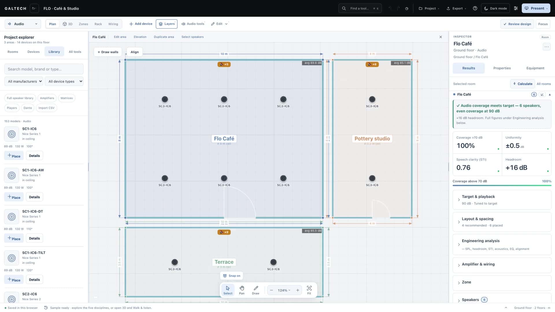
In a distributed system every speaker is a different distance from the listener, so their sound arrives at different times and blurs speech. Auto-align works out each speaker’s arrival time at the listening reference, the listener positions or the room centre, and stores a delay for each so that the arrivals land together: the farthest speaker gets 0 ms, the nearest the most.

Clear sets every delay back to 0. Use it in any area with two or more speakers where clarity matters, and always before you export the DSP preset. Each speaker’s delay can also be set by hand, in milliseconds, under Timing and alignment in its properties.

The DSP preset#

Export → DSP preset (PDF) produces a branded commissioning sheet for the processor. For every output it gives a full channel strip:

• a level trim and the polarity,
• high-pass and low-pass filters with their slope and type,
• the crossover for any zone with a subwoofer,
• a parametric EQ as a starting voicing, with a room-mode notch on subwoofers,
• a limiter set to the speaker’s rating,
• and the time-alignment delay.

It ends with a calibration walk sheet: every speaker’s number as on the plan, its position, height, aim, connection or tap, its level trim and its delay. Load it into the processor as your baseline, then verify and fine-tune on site with an SPL meter, and an STIPA check for speech.

Site calibration#

Site calibration turns the prediction into an as-built record. You measure the real average level after installation, and the tool shifts the whole model by the difference: the heatmap, the figures, the standards check and the walk-in all move to match the real room.

The offset shows on the card and is saved with the project; Clear returns to the raw prediction. Every calibrated area prints in the audio report as a Site Validation table, predicted against measured, so you build your own evidence of the model’s accuracy from project to project.

Site tracking#

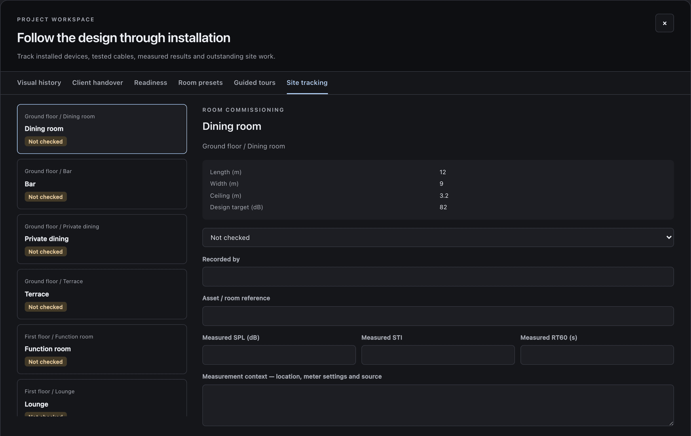
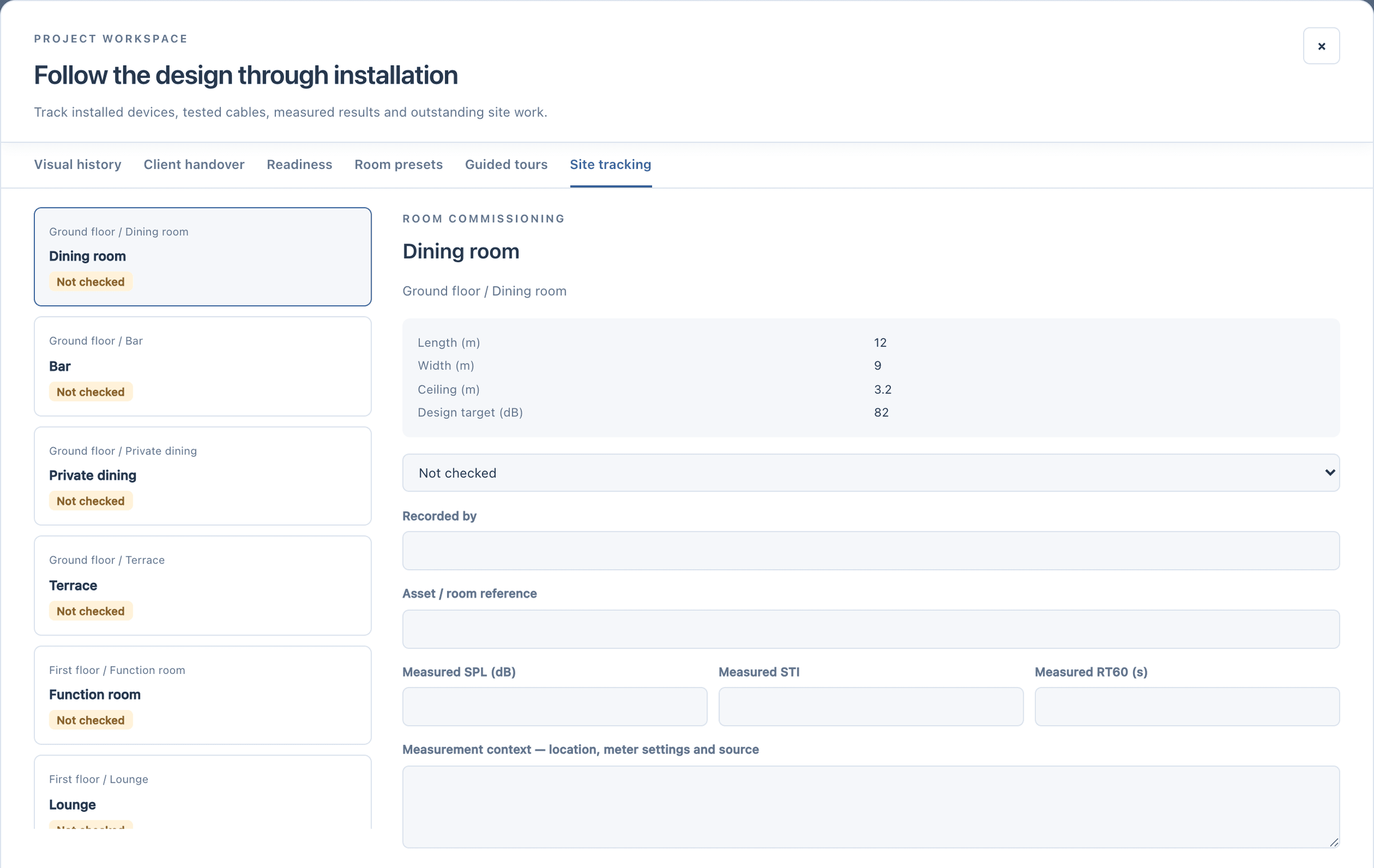
Site tracking follows the design through installation. Every device and every cable is an item with a status: not checked, installed, verified or needs attention, with who checked it and when. For each area you record the measured level, STI and RT60 next to what the tool predicted, and Export commissioning CSV gives you the record for the client’s file.